 Problem I. 290. (March 2012)
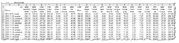
I. 290. Besides offering credit and managing deposits, banks also change and register various currencies. Fluctuating exchange rates strongly determine the commerce and economy of a country. In this task you are going to analyze some foreign exchange rates during the last two months of the last year by using data from the bank OTP. Exchange rates are updated during workdays, but this is complicated by the holidays and long weekends. Exchange rates on rest days are the same as the ones during the last working day before the rest day: exchange rates on October 28 are present in the table because the first day of November was a rest day.
Actual data are found in the tabulator separated UTF-8 encoded text file deviza.txt downloadable from our site.
Whenever possible, your solution should use formulae, functions and links. Auxiliary computations can be performed to the right of column V and below row 56.
[1.] Open the file deviza.txt in a spreadsheet application such that the first piece of data is put into cell A1. Save the sheet named i290 in the default file format of the application. The first two columns of the sheet contain the date and day of the week, the first row contains the currency codes, while the second row the currency names. Further rows contain the middle prices of the corresponding foreign currencies. For example, the value 348,58 (with comma denoting the decimal mark) in cell K28 means that on December 5, 2011 one GBP was equal to 348,58 HUF.
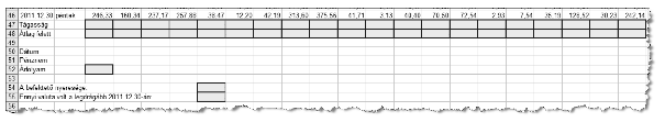
[2.] Range C47:V47 should contain the ratio between the highest and lowest value of the actual currency.
[3.] Range C48:V48 should contain the number of days during which the actual exchange rate was higher than its average. Rest days should be taken into account when counting days and computing the average.
[4.] On November 3, an investor bought (on middle prices) AUD, CAD and USD for 1 million HUF each. On December 19, the investor sold all the three types of dollars. The investor was charged 0.5% for the transactions. (In reality, banks use buying the selling rates when exchanging money, and the difference of these two is the profit of the bank. But for simplicity, we now use only middle prices and some additional charges.) Cell G54 should contain the profit of the investor. The format of the cell should be set to HUF currency without decimal digits.
[5.] Cell G55 should contain the number of currencies which attained their highest value on the last working day of the year (December 30, 2011).
[6.] You should create an expression in cell C52 which computes the actual exchange rate based on the values of cells C51 and C50, or displays an ``Invalid data'' message, if the corresponding data is missing (either the date is out of range or the currency is not in our list). For example, if 2011.11.17 is entered into cell C50 and NOK entered into cell C51, then cell C52 should display 39,39. If any of the two cells above is empty, cell C52 should remain empty, too. You should pay attention however, for example, for December 12, 2011 the valid exchange rate is known even if the original table does not contain it.
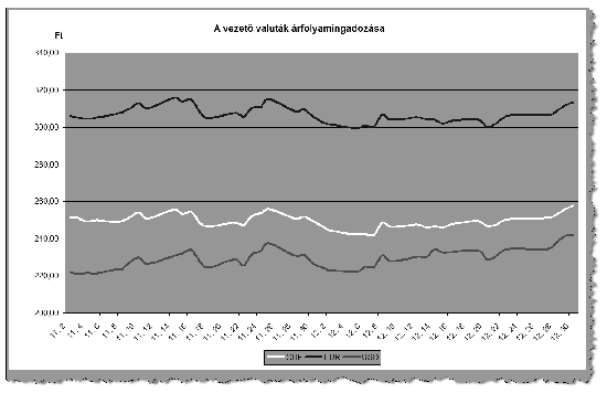
[7.] You should create a graph showing the fluctuating exchange rates for the USD, CHF and EUR during the whole period. You should consider the following.
\(\displaystyle a)\) The graph should show only data corresponding to working days.
\(\displaystyle b)\) The type of the graph should be line diagram.
\(\displaystyle c)\) The diagram should be created on a new sheet.
\(\displaystyle d)\) The rates for the USD should be displayed in thick red, the EUR in thick blue, while the CHF in thick white. The background and the legend should be dark enough so that the white curve is also properly visible.
\(\displaystyle e)\) The legend should be displayed below the diagram.
\(\displaystyle f)\) The title should be ``Fluctuations of the leading foreign currencies''.
\(\displaystyle g)\) The date should not contain the year. The scale on the vertical axis should range from 200 to 340, and Ft (that is, HUF) should be displayed on the top of that axis.
On the original sheet currency codes should be in bold face. These and the currency names should be centered in both directions. If necessary, the names can occupy more rows, according to the example. Range A1:B2 should be displayed as in the example.
[8.] Background color for cells with computed values should be pale green with dark green border.
Your spreadsheet (i290.xls, i290.ods, ...) together with a short documentation (i290.txt, i290.pdf, ...) should be submitted, also containing the name and version number of the spreadsheet application.
(10 pont)
Deadline expired on April 10, 2012.
Sorry, the solution is available only in Hungarian. Google translation
Antal János Benjámin (Nyíregyháza, Széchenyi I. Közg. Szki.) mintaszerű megoldását minden megoldó figyelmébe ajánlom. i290.xls
Statistics:
9 students sent a solution. 10 points: Antal János Benjamin. 9 points: Kalló Kristóf, Kovács Balázs Marcell, Kucsma Levente István. 8 points: 2 students. 7 points: 2 students. 5 points: 1 student.
Problems in Information Technology of KöMaL, March 2012